# Using functions in C++ - Pretty Plots

A good way to organize and structure computer programs is dividing them into smaller parts using functions. Each function carries out a specific task of the problem that we are solving.
You've seen that all programs written in C++ must contain the `main` function where the program begins. You've probably already used functions such as `pow`, `sin`, `cos`, or `sqrt` from the `cmath` library. Since in almost all of the upcoming lab experiences, you will continue using pre-defined functions, you need to understand how to work with them. In future exercises, you will learn how to design and prove functions. In this laboratory experience, you will call and define functions that compute the coordinates of the points of the graphs of some curves. You will also practice the implementation of arithmetic expressions in C++.
## Objectives:
1. Identify the parts of a function: return type, name, list of parameters, and body.
2. Call pre-defined functions by passing arguments by value ("pass by value"), and by reference ("pass by reference").
3. Implement a simple overloaded function.
4. Implement a simple function that utilizes parameters by reference.
5. Implement arithmetic expressions in C++.
## Pre-Lab:
Before you get to the laboratory you should have:
1. Reviewed the following concepts:
a. the basic elements of a function definition in C++.
b. how to call functions in C++.
c. the difference between parameters that are passed by value and by reference.
d. how to return the result of a function.
e. implement arithmetic expressions in C++.
f. use functions and arithmetic constants from the `cmath` library.
g. a circle's graph and equation.
2. Studied the concepts and instructions for the laboratory session.
3. Taken the Pre-Lab quiz, available in Moodle.
---
---
## Functions
In mathematics, a function $$f$$ is a rule that is used to assign to each element $$x$$ from a set called *domain*, one (and only one) element $$y$$ from a set called *range*. This rule is commonly represented with an equation, $$y=f(x)$$. The variable $$x$$ is the parameter of the function and the variable $$y$$ will contain the result of the function. A function can have more than one parameter, but only one result. For example, a function can have the form $$y=f(x_1,x_2)$$ where there are two parameters, and for each pair $$(a,b)$$ that is used as an argument in the function, the function will have only one value of $$y=f(a,b)$$. The domain of the function tells us the type of value that the parameter should have and the range tells us the value that the returned result will have.
Functions in programming languages are similar. A function has a series of instructions that take the assigned values as parameters and perform a certain task. In C++ and other programming languages, functions return only one result, as it happens in mathematics. The only difference is that a *programming* function could possibly not return any value (in this case the function is declared as `void`). If the function will return a value, we use the instruction `return`. As in math that you need to specify the domain and range, in programming you need to specify the types of values that the function's parameters and result will have; this is done when declaring the function.
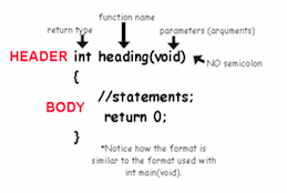
### Function Header
The first sentence of a function is called the *header* and its structure is as follows:
`type name(type parameter_1, ..., type parameter_n)`
For example,
`int example(int var1, float var2, char &var3)`
would be the header of the function called `example`, which returns an integer value. The function receives as arguments an integer value (and will store a copy in `var1`), a value of type `float` (and will store a copy in `var2`) and the reference to a variable of type `char` that will be stored in the reference variable `var3`. Note that `var3` has a & symbol before the name of the variable. This indicates that `var3` will contain the reference to a character.
### Calling
If we want to store the value of the result of the function called `example` in a variable `result` (that would be of type integer), we call the function by passing arguments as follows:
`result=example(2, 3.5, unCar);`
Note that as the function is called, you don't include the type of the variables in the arguments as in the definition for the function `example`. The third parameter `&var3` is a reference variable; this means that what is being sent to the third argument when invoking the function is a *reference* to the variable `unCar`. Any changes that are made on the variable `var3` will change the contents of the variable `unCar`.
You can also use the function's result without having to store it in a variable. For example you could print it:
`cout << "The result of the function example is:" << example(2, 3.5, unCar);`
or use it in an arithmetic expression:
`y = 3 + example(2, 3.5, unCar);`
### Overloaded Functions
Overloaded functions are functions that have the same name, but a different *signature*.
The signature of a function is composed of the name of the function, and the types of parameters it receives, but does not include the return type.
The following function prototypes have the same signature:
```
int example(int, int) ;
void example(int, int) ;
string example(int, int) ;
```
Note that each has the same name, `example`, and receives the same amount of parameters of the same type `(int, int)`.
The following function prototypes have different signatures:
```
int example(int) ;
int elpmaxe(int) ;
```
Note that even though the functions have the same amount of parameters with the same type `int`, the name of the functions is different.
The following function prototypes are overloaded versions of the function `example`:
```
int example(int) ;
void example(char) ;
int example(int, int) ;
int example(char, int) ;
int example(int, char) ;
```
All of the above functions have the same name, `example`, but different parameters. The first and second functions have the same amount of parameters, but their arguments are of different types. The fourth and fifth functions have arguments of type `char` and `int`, but have a different order in each case.
In that last example, the function `example` is overloaded since there are five functions with different signatures but with the same name.
### Default Values
Values by default can be assigned to the parameters of the functions starting from rightmost parameter. It is not necessary to initialize all of the parameters, but the ones that are initialized should be consecutive: parameters in between two parameters cannot be left uninitialized. This allows calling the function without having to send values in the positions that correspond to the initialized parameters.
**Examples of Function Headers and Valid Function Calls:**
1. **Header:** `int example(int var1, float var2, int var3 = 10)`
**Calls:**
a. `example(5, 3.3, 12)` This function call assigns the value 5 to `var1`, the value 3.3 to `var2`, and the value of 12 to `var3`.
b. `example(5, 3.3)` This function call sends the values for the first two parameters and the value for the last parameter will be the value assigned by default in the header. That is, the values in the variables in the function will be as follows: `var1` will be 5, `var2` will be 3.3, and `var3` will be 10.
2. **Header:** `int example(int var1, float var2=5.0, int var3 = 10)`
**Calls:**
a. `example(5, 3.3, 12)` This function call assigns the value 5 to `var1`, the value 3.3 to `var2`, and the value 12 to `var3`.
b. `example(5, 3.3)` In this function call only the first two parameters are given values, and the value for the last parameter is the value by default. That is, the value for `var1` within the function will be 5, that of `var2` will be 3.3, and `var3` will be 10.
c. `example(5)` In this function call only the first parameter is given a value, and the last two parameters will be assigned values by default. That is, `var1` will be 5, `var2` will be 5.0, and `var3` will be 10.
**Example of a Valid Function Header with Invalid Function Calls:**
1. **Header:** `int example(int var1, float var2=5.0, int var3 = 10)`
**Calls:**
a. `example(5, , 10)` This function call is **invalid** because it leaves an empty space in the middle argument.
b. `example()` This function call is **invalid** because `var1` was not assigned a default value. A valid call to function `example` needs at least one argument (the first).
**Examples of Invalid Function Headers:**
1. `int example(int var1=1, float var2, int var3)` This header is invalid because the default values can only be assigned starting from the rightmost parameter.
2. `int example(int var1=1, float var2, int var3=10)` This header is invalid because you can't place parameters without values between other parameters with default values. In this case, `var2` doesn't have a default value but `var1` and `var3` do.
---
---
## Parametric Equations
*Parametric equations* allow us to represent a quantity as a function of one or more independent variables called *parameters*. In many occasions it is useful to represent curves using a set of parametric equations that express the coordinates of the points of the curve as functions of the parameters. For example, in your trigonometry course you should have studied that the equation of the circle of radius $$r$$ and centered at the origin has the following form:
$$x^2+y^2=r^2.$$
The points $$(x,y)$$ that satisfy this equation are the points that form the circle of radius $$r$$ and center at the origin. For example, the circle with $$r=2$$ and center at the origin has equation
$$x^2+y^2=4,$$
and its points are the ordered pairs $$(x,y)$$ that satisfy this equation. A parametric representation of the coordinates of the points in the circle of radius $$r$$ and center at the origin is:
$$x=r \cos(t)$$
$$y=r \sin(t),$$
where $$t$$ is a parameter that corresponds to the measure (in radians) of the positive angle with an initial side that coincides with the positive part of the $$x$$-axis and a terminal side that contains the point $$(x,y)$$, as it is illustrated in Figure 1.
---
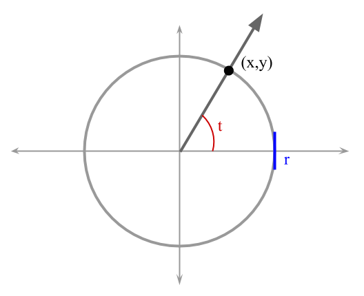
**Figure 1.** Circle with center in the origin and radius $$r$$.
---
To plot a curve that is described by parametric equations, we compute the $$x$$ and $$y$$ values for a set of values of the parameter. For example, Figure 2 shows the values for $$t$$, $$(x,y)$$ for the circle with $$r=2$$.
---
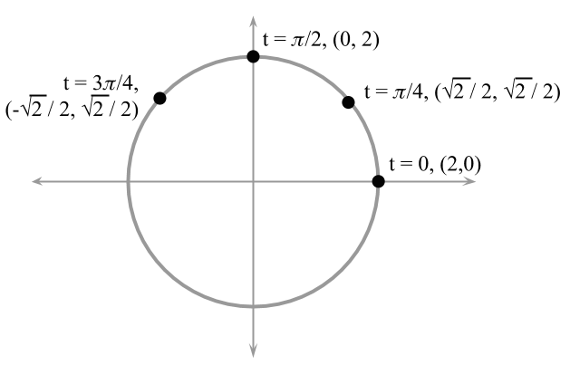
**Figure 2.** Some coordinates for the points $$(x,y)$$ for the circle with radius $$r=2$$ and center in the origin.
---
---
!INCLUDE "../../eip-diagnostic/DVD/en/diag-dvd-01.html"
!INCLUDE "../../eip-diagnostic/DVD/en/diag-dvd-03.html"
!INCLUDE "../../eip-diagnostic/DVD/en/diag-dvd-11.html"
!INCLUDE "../../eip-diagnostic/DVD/en/diag-dvd-12.html"
---
---
## Laboratory Session:
In the introduction to the topic of functions you saw that in mathematics and in some programming languages, a function cannot return more than one result. In this laboratory experience's exercises, you will practice how to use reference variables to obtain various results from a function.
### Exercise 1 - Difference between Pass by Value and Pass by Reference
#### Instructions
1. Load the project ‘prettyPlot’ into ‘QtCreator`. There are two ways to do this:
* Using the virtual machine: Double click the file `prettyPlot.pro` located in the folder `home/eip/labs/functions-prettyplots` of your virtual machine.
* Downloading the project’s folder from `Bitbucket`: Use a terminal and write the command `git clone http://bitbucket.org/eip-uprrp/functions-prettyplots` to download the folder `functions-prettyplots` from `Bitbucket`. Double click the file `prettyPlot.pro` located in the folder that you downloaded to your computer.
2. Configure the project and execute the program by clicking on the green arrow in the menu on the left side of the Qt Creator screen. The program should show a window similar to the one in Figure 3.
---
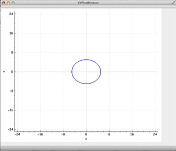
**Figure 3.** Graph of a circle with radius 5 and center in the origin displayed by the program *PrettyPlot*.
---
3. Open the file `main.cpp` (in Sources). Study the `illustration` function and how to call it from the `main` function. Note that the variables `argValue` and `argRef`are initialized to 0 and that the function call for `illustration` makes a pass by value of `argValue` and a pass by reference of `argRef`. Also note that the corresponding parameters in `illustration` are assigned a value of 1.
void illustration(int paramValue, int ¶mRef) {
paramValue = 1;
paramRef = 1;
cout << endl << "The content of paramValue is: " << paramValue << endl
<< "The content of paramRef is: " << paramRef << endl;
}
4. Execute the program and observe what is displayed in the window `Application Output`. Notice the difference between the content of the variables `argValue` and `argRef` despite the fact that both had the same initial value, and that `paramValue` and `paramRef` were assigned the same value. Explain why the content of `argValor` does not change, while the content of `argRef` changes from 0 to 1.
### Exercise 2 - Creation of an Overloaded Function
#### Instructions
1. Study the code in the `main()` function in the file `main.cpp`. The line `XYPlotWindow wCircleR5;` creates a `wCircleR5` object that will be the window where the graph will be drawn, in this case the graph of a circle of radius 5. In a similar way, the objects `wCircle` and `wButterfly` are created. Observe the `for` cycle. In this cycle a series of values for the angle $$t$$ are generated and the function `circle` is called, passing the value for $$t$$ and the references to $$x$$ and $$y$$. The `circle` function does not return a value, but by using parameters by reference, it calculates the values for the coordinates $$xCoord$$ and $$yCoord$$ for the circle with center in the origin and radius 5, and allows the `main` function to have these values in the `x` , `y` variables.
XYPlotWindow wCircleR5;
XYPlotWindow wCircle;
XYPlotWindow wButterfly;
double r;
double y = 0.00;
double x = 0.00;
double increment = 0.01;
int argValue=0, argRef=0;
// call the function illustration to view the contents of variables
// by value and by reference
illustration(argValue,argRef);
cout << endl << "The content of argValue is: " << argValue << endl
<< "The content of argRef is: " << argRef << endl;
// repeat for several values of the angle t
for (double t = 0; t < 16*M_PI; t = t + increment) {
// call circle with the angle t and reference variables x, y as arguments
circle(t,x,y);
// add the point (x,y) to the graph of the circle
wCircleR5.AddPointToGraph(x,y);
}
After the function call, each ordered pair $$(x,y)$$ is added to the circle’s graph by the member function `AddPointToGraph(x,y)`. After the cycle, the member function `Plot()` is called, which draws the points, and the member function `show()`, which displays the graph. The *member functions* are functions that allow us to work with an object’s data. Notice that each one of the member functions is written after `wCircleR5`, followed by a period. In an upcoming laboratory experience you will learn more about objects, and practice how to create them and invoke their method functions.
The `circle` function implemented in the program is very restrictive since it always calculates the values for the coordinates $$x$$ and $$y$$ of the same circle: the circle with center in the origin and radius 5.
2. Now you will create an overloaded function `circle` that receives as arguments the value of the angle $$t$$, the reference to the variables $$x$$ and $$y$$, and the value for the radius of the circle. Call the overloaded function `circle` that you just implemented from `main()` to calculate the values of the coordinates $$x$$ and $$y$$ for the circle with radius 15 and draw its graph. Graph the circle within the `wCircle` object. To do this, you must call the method functions `AddPointToGraph(x,y)`, `Plot` and `show` from `main()`. Remember that these should be preceded by `wCircle`, for example, `wCircle.show()`.
### Exercise 3 - Implement a Function to Calculate the Coordinates of the Points in the Graph of a Curve
#### Instructions
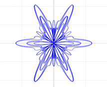
1. Now you will create a function to calculate the coordinates of the points of a graph that resembles a butterfly. The parametric equations for the coordinates of the points in the graph are given by:
$$x=5\cos(t) \left[ \sin^2(1.2t) + \cos^3(6t) \right]$$
$$y= 10\sin(t) \left[ \sin^2(1.2t) + \cos^3(6t) \right].$$
Observe that both expressions are almost the same, except that one starts with $$5\cos(t)$$ and the other with $$10\sin(t)$$. Instead of doing the calculation for $$ \sin^2(1.2t) + \cos^3(6t)$$ twice, you can assign its value to another variable $$q$$ and calculate it as such:
$$q = \sin^2(1.2t) + \cos^3(6t)$$
$$x = 5 \cos(t)(q)$$
$$y = 10 \sin(t)(q).$$
2. Implement the function `butterfly` using the expressions above, call the function in `main()` and observe the resulting graph. It is supposed to look like a butterfly. This graph should have been obtained with a `XYPlotWindow` object called `wButterfly`, invoking method functions similar to how you did in Exercise 2 for the circle.
In [2] and [3] you can find other parametric equations from other interesting curves.
---
---
##Deliverables
Use "Deliverables" in Moodle to hand in the file `main.cpp` that contains the functions you implemented, the function calls and changes you made in exercises 2 and 3. Remember to use good programming techniques, include the name of the programmers involved and document your program.
---
---
##References
[1] http://mathbits.com/MathBits/CompSci/functions/UserDef.htm
[2] http://paulbourke.net/geometry/butterfly/
[3] http://en.wikipedia.org/wiki/Parametric_equation