
 Jose Ortiz
4d4df27b96
Changes to the source files
Jose Ortiz
4d4df27b96
Changes to the source files
|
10 years ago | |
|---|---|---|
| doc | 10 years ago | |
| images | 10 years ago | |
| README.md | 10 years ago | |
| main.cpp | 10 years ago | |
| prettyPlot.pro | 10 years ago | |
| qcustomplot.cpp | 10 years ago | |
| qcustomplot.h | 10 years ago | |
| xyplotwindow.cpp | 10 years ago | |
| xyplotwindow.h | 10 years ago | |
| xyplotwindow.ui | 10 years ago |
README.md
Expresiones aritméticas - Gráficas Bonitas

Las expresiones aritméticas son parte esencial de casi cualquier algoritmo que resuelve un problema útil. Por lo tanto, implementar expresiones aritméticas correctamente es una destreza básica en cualquier lenguaje de programación de computadoras. En esta experiencia de laboratorio practicarás la implementación de expresiones aritméticas en C++ escribiendo ecuaciones paramétricas para graficar curvas interesantes.
Objetivos:
- Implementar expresiones aritméticas en C++ para producir gráficas.
- Utilizar constantes adecuadamente.
- Definir variables utilizando tipos de datos adecuados.
- Convertir el valor de un dato a otro tipo cuando sea necesario.
Pre-Lab:
Antes de llegar al laboratorio debes:
Haber repasado los siguientes conceptos:
a. implementar expresiones aritméticas en C++
b. tipos de datos nativos de C++ (int, float, double, char)
c. usar “type casting” para covertir el valor de una variable a otro tipo dentro de expresiones.
d. utilizar funciones y constantes aritméticas de la biblioteca
cmathe. la ecuación y gráfica de un círculo
Haber estudiado los conceptos e instrucciones para la sesión de laboratorio.
Haber tomado el quiz Pre-Lab que se encuentra en Moodle.
Ecuaciones paramétricas
Las ecuaciones paramétricas nos permiten representar una cantidad como función de una o más variables independientes llamadas parámetros. En muchas ocasiones resulta útil representar curvas utilizando un conjunto de ecuaciones paramétricas que expresen las coordenadas de los puntos de la curva como funciones de los parámetros. Por ejemplo, en tu curso de trigonometría debes haber estudiado que la ecuación de un círculo con radio $$r$$ y centro en el origen tiene una forma así:
$$x^2+y^2=r^2.$$
Los puntos $$(x,y)$$ que satisfacen esta ecuación son los puntos que forman el círculo de radio $$r$$ y centro en el origen. Por ejemplo, el círculo con $$r=2$$ y centro en el origen tiene ecuación
$$x^2+y^2=4,$$
y sus puntos son los pares ordenados $$(x,y)$$ que satisfacen esa ecuación. Una forma paramétrica de expresar las coordenadas de los puntos de el círculo con radio $$r$$ y centro en el origen es:
$$x=r \cos(t)$$
$$y=r \sin(t),$$
donde $$t$$ es un parámetro que corresponde a la medida (en radianes) del ángulo positivo con lado inicial que coincide con la parte positiva del eje de $$x$$, y lado terminal que contiene el punto $$(x,y)$$, como se muestra en la Figura 1.
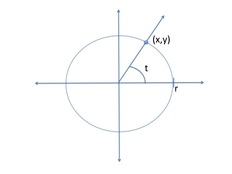
Figura 1. Círculo con centro en el origen y radio $$r$$.
Para graficar una curva que está definida usando ecuaciones paramétricas, computamos los valores de $$x$$ y $$y$$ para un conjunto de valores del parámetro. Por ejemplo, para $$r = 2$$, algunos de los valores son
| $$t$$ | $$x$$ | $$y$$ |
|---|---|---|
| $$0$$ | $$2$$ | $$0$$ |
| $$\frac{\pi}{4}$$ | $$\frac{\sqrt{2}}{2}$$ | $$\frac{\sqrt{2}}{2}$$ |
| $$\frac{\pi}{2}$$ | $$0$$ | $$2$$ |
Figura 2. Algunas coordenadas de los puntos $$(x,y)$$ del círculo con radio $$r=2$$ y centro en el origen.
!INCLUDE “../../eip-diagnostic/pretty-plots/es/diag-pretty-plots-01.html”
!INCLUDE “../../eip-diagnostic/pretty-plots/es/diag-pretty-plots-02.html”
!INCLUDE “../../eip-diagnostic/pretty-plots/es/diag-pretty-plots-03.html”
!INCLUDE “../../eip-diagnostic/pretty-plots/es/diag-pretty-plots-04.html”
Sesión de laboratorio:
Ejercicio 1
En este ejercicio graficarás algunas ecuaciones paramétricas que generan curvas interesantes.
Instrucciones
Carga a Qt el proyecto
prettyPlothaciendo doble “click” en el archivoprettyPlot.proque se encuentra en la carpetaDocuments/eip/Expressions-PrettyPlotsde tu computadora. También puedes ir ahttp://bitbucket.org/eip-uprrp/expressions-prettyplotspara descargar la carpetaExpressions-PrettyPlotsa tu computadora.Configura el proyecto y ejecuta el programa marcando la flecha verde en el menú de la izquierda de la ventana de Qt Creator. El programa debe mostrar una ventana parecida a la Figura 3.

Figura 3. Segmento de línea desplegado por el programa PrettyPlot.
El archivo
main.cpp(en Sources) contiene la funciónmain()donde estarás añadiendo código. Abre ese archivo y estudia el código. La líneaXYPlotWindow wLine;crea el objetowLineque será la ventana en donde se dibujará una gráfica, en este caso la gráfica de un segmento. Observa el ciclofor. En este ciclo se genera una serie de valores para $$t$$ y se computa un valor de $$x$$ y $$y$$ para cada valor de $$t$$. Cada par ordenado $$(x,y)$$ es añadido a la gráfica del segmento por el métodoAddPointToGraph(x,y). Luego del ciclo se invoca el métodoPlot(), que “dibuja” los puntos, y el métodoshow(), que muestra la gráfica. Los métodos son funciones que nos permiten trabajar con los datos de los objetos. Nota que cada uno de los métodos se escribe luego dewLine, seguido de un punto. En una experiencia de laboratorio posterior aprenderás más sobre objetos y practicarás como crearlos e invocar sus métodos.Las expresiones que tiene tiene tu programa para $$x$$ y $$y$$ son ecuaciones paramétricas para la línea que pasa por el origen y tiene el mismo valor para las coordenadas en $$x$$ y $$y$$. Explica por qué la línea solo va desde 0 hasta aproximadamente 6.
Ahora escribirás el código necesario para graficar un círculo. La línea
XYPlotWindow wCircle;crea el objetowCirclepara la ventana donde se graficará el círculo. Usando como inspiración el código para graficar el segmento, escribe el código necesario para que tu programa grafique un círculo de radio 3 con centro en el origen. Ejecuta tu programa y, si es necesario, modifica el código hasta que obtengas la gráfica correcta. Recuerda que el círculo debe graficarse dentro del objetowCircle. Por esto, al invocar los métodosAddPointToGraph(x,y),Plotyshow, éstos deben ser precedidos porwCircle, por ejemplo,wCircle.show().Tu próxima tarea es graficar una curva cuyas ecuaciones paramétricas son:
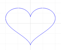
$$x=16 \sin^3(t)$$ $$y=13 \cos(t) - 5 \cos(2t) - 2 \cos(3t) - \cos(4t)-3.$$
Si implementas las expresiones correctamente debes ver la imagen de un corazón. Esta gráfica debe haber sido obtenida dentro de un objeto
XYPlotWindowllamadowHeart.Ahora graficarás una curva cuyas ecuaciones paramétricas son:
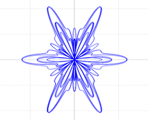
$$x=5\cos(t) \left[ \sin^2(1.2t) + \cos^3(6t) \right]$$ $$y= 10\sin(t) \left[ \sin^2(1.2t) + \cos^3(6t) \right].$$
Observa que ambas expresiones son casi iguales, excepto que una comienza con $$5\cos(t)$$ y la otra con $$10\sin(t)$$. En lugar de realizar el cómputo de $$ \sin^2(1.2t) + \cos^3(6t)$$ dos veces, puedes asignar su valor a otra variable $$q$$ y realizar el cómputo así:
$$q = \sin^2(1.2t) + \cos^3(6t)$$ $$x = 5 \cos(t)(q)$$ $$y = 10 \sin(t)(q).$$
Implementa las expresiones de arriba, cambia la condición de terminación del
forat < 16*M_PIy observa la gráfica que resulta. Se supone que parezca una mariposa. Esta gráfica debe haber sido obtenida dentro de un objetoXYPlotWindowllamadowButterfly.Entrega el archivo
main.cppque contiene el código con las ecuaciones paramétricas de las gráficas del círculo, el corazón y la mariposa utilizando “Entrega 1” en Moodle. Recuerda utilizar buenas prácticas de programación, incluir el nombre de los programadores y documentar tu programa.
En [3] puedes encontrar otras ecuaciones paramétricas de otras curvas interesantes.
Ejercicio 2
En este ejercicio escribirás un programa para obtener el promedio de puntos para la nota de un estudiante.
Supón que todos los cursos en la Universidad de Yauco son de $$3$$ créditos y que las notas tienen las siguientes puntuaciones: $$A = 4$$ puntos por crédito; $$B = 3$$ puntos por crédito; $$C = 2$$ puntos por crédito; $$D = 1$$ punto por crédito y $$F = 0$$ puntos por crédito.
!INCLUDE “../../eip-diagnostic/pretty-plots/es/diag-pretty-plots-05.html”
!INCLUDE “../../eip-diagnostic/pretty-plots/es/diag-pretty-plots-06.html”
!INCLUDE “../../eip-diagnostic/pretty-plots/es/diag-pretty-plots-07.html”
Instrucciones
Crea un nuevo proyecto “Non-Qt” llamado Promedio. Tu función
main()contendrá el código necesario para pedirle al usuario el número de A’s, B’s, C’s, D’s y F’s obtenidas por el estudiante y computar el promedio de puntos para la nota (GPA por sus siglas en inglés).Tu código debe definir las constantes $$A=4, B=3, C=2, D=1, F=0$$ para la puntuación de las notas, y pedirle al usuario que entre los valores para las variables $$NumA$$, $$NumB$$, $$NumC$$, $$NumD$$, $$NumF$$. La variable $$NumA$$ representará el número de cursos en los que el estudiante obtuvo $$A$$, $$NumB$$ representará el número de cursos en los que el estudiante obtuvo $$B$$, etc. El programa debe desplegar el GPA del estudiante en una escala de 0 a 4 puntos.
Ayudas:
El promedio se obtiene sumando las puntuaciones correspondientes a las notas obtenidas (por ejemplo, una A en un curso de 3 créditos tiene una puntuación de 12), y dividiendo esa suma por el número total de créditos.
Recuerda que, en C++, si divides dos números enteros el resultado se “truncará” y será un número entero. Utiliza “type casting”: `static_cast<tipo>(expresión)’ para resolver este problema.
Verifica tu programa calculando el promedio de un estudiante que tenga dos A y dos B; ¿qué nota tendría este estudiante, A o B (la A va desde 3.5 a 4.0)?. Cuando tu programa esté correcto, guarda el archivo
main.cppy entrégalo utilizando “Entrega 2” en Moodle. Recuerda seguir las instrucciones en el uso de nombres y tipos para las variables, incluir el nombre de los programadores, documentar tu programa y utilizar buenas prácticas de programación.
Referencias:
[1] http://mathworld.wolfram.com/ParametricEquations.html
[2] http://paulbourke.net/geometry/butterfly/
[3] http://en.wikipedia.org/wiki/Parametric_equation
Arithmetic Expressions - Pretty Plots
Arithmetic expressions are an essential part of almost any algorithm that solves a useful problem. Therefore, a basic skill in any computer programming language is to implement arithmetic expressions correctly. In this laboratory experience you will practice the implementation of arithmetic expressions in C++ by writing parametric equations to plot interesting curves.
Objectives:
- To implement arithmetic expressions in C++ to produce graphs.
- To use constants adequately.
- To define variables using adequate data types.
- To cast a data value to another type when necessary.
Pre-Lab:
Before you get to the laboratory you should have:
Reviewed the following concepts:
a. implementing arithmetic expressions in C++.
b. native data types in C++ (int, float, double)
c. using “type casting” to cast the value of variables to other data types within expressions.
d. using arithmetic functions and constants from the
cmathlibrary.e. the equation and graph of a circle.
Studied the concepts and instructions for the laboratory session.
Taken the Pre-Lab quiz that can be found in Moodle.
Parametric Equations
Parametric equations allow us to represent a quantity as a function of one or more independent variables called parameters. In many occasions it is useful to represent curves using a set of parametric equations that express the coordinates of the points of the curve as functions of the parameters. For example, in your trigonometry course you should have studied that the equation of the circle of radius $$r$$ and centered at the origin has the following form:
$$x^2+y^2=r^2.$$
The points $$(x,y)$$ that satisfy this equation are the points that form the circle of radius $$r$$ and center at the origin. For example, the circle with $$r=2$$ and center at the origin has equation
$$x^2+y^2=4,$$
and its points are the ordered pairs $$(x,y)$$ that satisfy this equation. A parametric representation of the coordinates of the points in the circle of radius $$r$$ and center at the origin is:
$$x=r \cos(t)$$
$$y=r \sin(t),$$
where $$t$$ is a parameter that corresponds to the measure (in radians) of the positive angle with initial side that coincides with the positive part of the $$x$$-axis and terminal side that contains the point $$(x,y)$$, as it is illustrated in Figure 1.
Figure 1. Circle of radius $$r$$ and centered at the origin.
To plot a curve that is described by parametric equations, we compute the $$x$$ and $$y$$ values for a set of values of the parameter. For example, for $$r=2$$, some of the values are
| $$t$$ | $$x$$ | $$y$$ |
|---|---|---|
| $$0$$ | $$2$$ | $$0$$ |
| $$\frac{\pi}{4}$$ | $$\frac{\sqrt{2}}{2}$$ | $$\frac{\sqrt{2}}{2}$$ |
| $$\frac{\pi}{2}$$ | $$0$$ | $$2$$ |
Figure 2. Some of the coordinates of the points $$(x,y)$$ of the circle of radius $$r=2$$ and centered at the origin.
!INCLUDE “../../eip-diagnostic/pretty-plots/en/diag-pretty-plots-01.html”
!INCLUDE “../../eip-diagnostic/pretty-plots/en/diag-pretty-plots-02.html”
!INCLUDE “../../eip-diagnostic/pretty-plots/en/diag-pretty-plots-03.html”
!INCLUDE “../../eip-diagnostic/pretty-plots/en/diag-pretty-plots-04.html”
Laboratory session:
Exercise 1
In this exercise you will plot the graphs of some parametric equations of interesting curves.
Instructions
Double click the file
prettyPlot.prothat is inside theDocuments/eip/Expressions-PrettyPlotsfolder to load the projectprettyPlotinto Qt. You can also download the folderExpressions-PrettyPlotsfromhttp://bitbucket.org/eip-uprrp/expressions-prettyplots.Configure the project and run the program by clicking the green arrow in the menu on the left side of the Qt Creator window. The program should display a window similar to the one in Figure 3.
Figure 3. Line segment displayed by the program PrettyPlot.
The file
main.cpp(in Sources) contains the functionmain()where you will be adding code. Open this file and study the code. The lineXYPlotWindow wLine;creates the objectwLine, that is the window that will show the plot of a graph, in this case the graph of a segment. Look at theforcycle. In this cycle several values for $$t$$ are generated and a value for $$x$$ and $$y$$ is computed for each $$t$$. Each ordered pair $$(x,y)$$ is added to the graph of the segment by the methodAddPointToGraph(x,y). After the cycle, there is a call to the methodPlot(), to “draw” the points in the graph, and to the methodshow(), to show the plot. The methods are functions that allow us to work with the data of an object. Note that each of the methods is written afterwLine, and followed by a period. In a later laboratory experience you will learn more about objects and practice how to create them and invoke their methods.The expressions for $$x$$ and $$y$$ are parametric equations for the line that passes through the origin and has the same value for $$x$$ and $$y$$. Explain why this line only goes from 0 to approximately 6.
You will now write the code needed to plot a circle. The line
XYPlotWindow wCircle;creates the objectwCirclefor the window that will contain the plot of the circle. Using as inspiration the code that plotted the segment, write the necessary code for your program to graph a circle of radius 3 and centered at the origin. Run your program and, if it is necessary, modify the code until you get the right plot. Remember that the circle should be plotted inside thewCircleobject. Thus, when you invoke theAddPointToGraph(x,y),Plotandshowmethods, they should be preceeded bywCircle; e.g.wCircle.show().Your next task is to plot a curve with the following parametric equations:
$$x=16 \sin^3(t)$$ $$y=13 \cos(t) - 5 \cos(2t) - 2 \cos(3t) - \cos(4t)-3.$$
If you implement the equations correctly, you will see the image of a heart. This plot should be obtained inside an
XYPlotWindowobject calledwHeart.You will now plot the curve of the following parametric equations:
$$x=5\cos(t) \left[ \sin^2(1.2t) + \cos^3(6t) \right]$$ $$y= 10\sin(t) \left[ \sin^2(1.2t) + \cos^3(6t) \right].$$
Note that both expressions are almost the same, the only difference is that one starts with $$5\cos(t)$$ and the other with $$10\sin(t)$$. Instead of computing $$\sin^2(1.2t) + \cos^3(6t)$$ twice, you can assign its value to another variable $$q$$ and compute $$x$$ and $$y$$ as follows:
$$q = \sin^2(1.2t) + \cos^3(6t)$$ $$x = 5 \cos(t)(q)$$ $$y = 10 \sin(t)(q).$$
Implement the above expressions, change the condition for termination of the
fortot < 16*M_PI, and look at the plot that it is displayed. It should look like a butterfly. This plot should be obtained inside anXYPlotWindowobject calledwButterfly.Use “Deliverable 1” in Moodle to submit the file
main.cppcontaining the code with the parametric equations for the graphs of the circle, the heart, and the butterfly. Remember to use good programming practices, to include the names of the programmers and to document your program.
In [3] you can find other parametric equations of interesting curves.
Exercise 2
In this exercise you will write a program to obtain a student’s grade point average (GPA).
Suppose that all courses in Cheo’s University are 3 credits each and have the following point values: $$A = 4$$ points per credit; $$B = 3$$ points per credit; $$C = 2$$ points per credit; $$D = 1$$ point per credit y $$F = 0$$ points per credit.
!INCLUDE “../../eip-diagnostic/pretty-plots/en/diag-pretty-plots-05.html”
!INCLUDE “../../eip-diagnostic/pretty-plots/en/diag-pretty-plots-06.html”
!INCLUDE “../../eip-diagnostic/pretty-plots/en/diag-pretty-plots-07.html”
Instructions
Start a new “Non-Qt” project called “Average”. Your
main()function will contain the necessary code to ask the user for the number of A’s, B’s, C’s, D’s and F’s obtained and compute the grade point average (GPA).Your code should define the constants $$A=4, B=3, C=2, D=1, F=0$$ for the points per credit, and ask the user to input the values for the variables $$NumA$$, $$NumB$$, $$NumC$$, $$NumD$$, $$NumF$$. The variable $$NumA$$ represents the number of courses in which the student obtained A, $$NumB$$ represents the number of courses in which the student obtained B, etc. The program should display the GPA using the 0-4 point scale.
Hints:
You can obtain the GPA by adding the credit points corresponding to the grades (for example, an A in a 3 credit course has a value of 12 points), and dividing this sum by the total number of credits.
Remember that, in C++, when both operands in the division are integers, the result will also be an integer; the remainder will be discarded. Use “type casting”: `static_cast<type>(expression)’ to solve this problem.
Verify your program by computing the GPA of a student that has two A’s and 2 B’s; what is the grade of this student, A or B (A goes from 3.5 to 4 points)? When your program is correct, save the
main.cppfile and submit it using “Deliverable 2” in Moodle. Remember to follow the instructions regarding the names and types of the variables, to include the names of the programmers, to document your program and to use good programming practices.
References:
[1] http://mathworld.wolfram.com/ParametricEquations.html