
 Jose Ortiz
ad0f8e46a7
Pretty Plots functions no sol initial commit
Jose Ortiz
ad0f8e46a7
Pretty Plots functions no sol initial commit
|
10 years ago | |
|---|---|---|
| doc | 10 years ago | |
| images | 10 years ago | |
| README.md | 10 years ago | |
| main.cpp | 10 years ago | |
| prettyPlot.pro | 10 years ago | |
| qcustomplot.cpp | 10 years ago | |
| qcustomplot.h | 10 years ago | |
| xyplotwindow.cpp | 10 years ago | |
| xyplotwindow.h | 10 years ago | |
| xyplotwindow.ui | 10 years ago |
README.md
Utilizando funciones en C++ - Gráficas Bonitas

Una buena manera de organizar y estructurar los programas de computadoras es dividiéndolos en partes más pequeñas utilizando funciones. Cada función realiza una tarea específica del problema que estamos resolviendo.
Haz visto que todos los programas en C++ deben contener la función main que es donde comienza el programa. Probablemente ya haz utilizado funciones como pow, sin, cos o sqrt de la biblioteca de matemática cmath. Dado que en casi todas las experiencias de laboratorio futuras estarás utilizando funciones que ya han sido creadas, necesitas aprender cómo trabajar con ellas. Más adelante aprenderás cómo diseñarlas y validarlas. En esta experiencia de laboratorio invocarás y definirás funciones que calculan las coordenadas de los puntos de las gráficas de algunas curvas. También practicarás la implementación de expresiones aritméticas en C++.
Objetivos:
- Identificar las partes de una función: tipo, nombre, lista de parámetros y cuerpo de la función.
- Invocar funciones ya creadas enviando argumentos por valor (“pass by value”) y por referencia (“pass by reference”).
- Implementar una función sobrecargada simple.
- Implementar funciones simples que utilicen parámetros por referencia.
- Implementar expresiones aritméticas en C++
Pre-Lab:
Antes de llegar al laboratorio debes:
Haber repasado los siguientes conceptos:
a. los elementos básicos de la definición de una función en C++.
b. la manera de invocar funciones en C++.
c. la diferencia entre parámetros pasados por valor y por referencia.
d. como devolver el resultado de una función.
e. implementar expresiones aritméticas en C++.
f. utilizar funciones y constantes aritméticas de la biblioteca
cmath.g. la ecuación y gráfica de un círculo.
Haber estudiado los conceptos e instrucciones para la sesión de laboratorio.
Haber tomado el quiz Pre-Lab que se encuentra en Moodle.
Funciones
En matemática, una función $f$ es una regla que se usa para asignar a cada elemento $x$ de un conjunto que se llama dominio, uno (y solo un) elemento $y$ de un conjunto que se llama campo de valores. Por lo general, esa regla se representa como una ecuación, $y=f(x)$. La variable $x$ es el parámetro de la función y la variable $y$ contendrá el resultado de la función. Una función puede tener más de un parámetro pero solo un resultado. Por ejemplo, una función puede tener la forma $y=f(x_1,x_2)$ en donde hay dos parámetros y para cada par $(a,b)$ que se use como argumento de la función, la función tiene un solo valor de $y=f(a,b)$. El dominio de la función te dice el tipo de valor que debe tener el parámetro y el campo de valores el tipo de valor que tendrá el resultado que devuelve la función.
Las funciones en lenguajes de programación de computadoras son similares. Una función
tiene una serie de instrucciones que toman los valores asignados a los parámetros y realiza alguna tarea. En C++ y en algunos otros lenguajes de programación, las funciones solo pueden devolver un resultado, tal y como sucede en matemáticas. La única diferencia es que una función en programación puede que no devuelva valor (en este caso la función se declara void). Si la función va a devolver algún valor, se hace con la instrucción return. Al igual que en matemática tienes que especificar el dominio y el campo de valores, en programación tienes que especificar los tipos de valores que tienen los parámetros y el resultado que devuelve la función; esto lo haces al declarar la función.
Encabezado de una función:
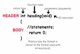
La primera oración de una función se llama el encabezado y su estructura es como sigue:
tipo nombre(tipo parámetro01, ..., tipo parámetro0n)
Por ejemplo,
int ejemplo(int var1, float var2, char &var3)
sería el encabezado de la función llamada ejemplo, que devuelve un valor entero. La función recibe como argumentos un valor entero (y guardará una copia en var1), un valor de tipo float (y guardará una copia en var2) y la referencia a una variable de tipo char que se guardará en la variable de referencia var3. Nota que var3 tiene el signo & antes del nombre de la variable. Esto indica que var3 contendrá la referencia a un caracter.
Invocación
Si queremos guardar el valor del resultado de la función ejemplo en la variable resultado (que deberá ser de tipo entero), invocamos la función pasando argumentos de manera similar a:
resultado=ejemplo(2, 3.5, unCar);
Nota que al invocar funciones no incluyes el tipo de las variables en los argumentos. Como en la definición de la función ejemplo el tercer parámetro &var3 es una variable de referencia, lo que se está enviando en el tercer argumento de la invocación es una referencia a la variable unCar. Los cambios que se hagan en la variable var3 están cambiando el contenido de la variable unCar.
También puedes usar el resultado de la función sin tener que guardarlo en una variable. Por ejemplo puedes imprimirlo:
cout << "El resultado de la función ejemplo es:" << ejemplo(2, 3.5, unCar);
o utilizarlo en una expresión aritmética:
y=3 + ejemplo(2, 3.5, unCar);
Funciones sobrecargadas (‘overloaded’)
Las funciones sobrecargadas son funciones que poseen el mismo nombre, pero firma diferente.
La firma de una función se compone del nombre de la función, y los tipos de parámetros que recibe, pero no incluye el tipo que devuelve.
Los siguientes prototipos de funciones tienen la misma firma:
int ejemplo(int, int) ;
void ejemplo(int, int) ;
string ejemplo(int, int) ;
Nota que todas tienen el mismo nombre, ejemplo, y reciben la misma cantidad de parámetros del mismo tipo (int, int).
Los siguientes prototipos de funciones tienen firmas diferentes:
int ejemplo(int) ;
int olpmeje(int) ;
Nota que a pesar de que las funciones tienen la misma cantidad de parámetros con mismo tipo int, el nombre de las funciones es distinto.
Los siguientes prototipos de funciones son versiones sobrecargadas de la función ejemplo:
int ejemplo(int) ;
void ejemplo(char) ;
int ejemplo(int, int) ;
int ejemplo(char, int) ;
int ejemplo(int, char) ;
Todas las funciones de arriba tienen el mismo nombre, ejemplo, pero distintos parámetros. La primera y segunda función tienen la misma cantidad de parámetros, pero los argumentos son de distintos tipos. La cuarta y quinta función tienen argumentos de tipo char e int, pero en cada caso están en distinto orden.
En este último ejemplo la función ejemplo es sobrecargada ya que hay 5 funciones con firma distinta pero con el mismo nombre.
Valores por defecto
Se pueden asignar valores por defecto (“default”) a los parámetros de las funciones comenzando desde el parámetro más a la derecha. No hay que inicializar todos los parámetros pero los que se inicializan deben ser consecutivos: no se puede dejar parámetros sin inicializar entre dos parámetros que estén inicializados. Esto permite la invocación de la función sin tener que enviar los valores en las posiciones que corresponden a parámetros inicializados.
Ejemplos de encabezados de funciones e invocaciones válidas:
Encabezado:
int ejemplo(int var1, float var2, int var3 = 10)Aquí se inicializavar3a 10.Invocaciones:
a.
ejemplo(5, 3.3, 12)Esta invocación asigna el valor 5 avar1, el valor 3.3 avar2, y el valor 12 avar3.b.
ejemplo(5, 3.3)Esta invocación envía valores para los primeros dos parámetros y el valor del último parámetro será el valor por defecto asignado en el encabezado. Esto es, los valores de las variables en la función serán:var1tendrá 5,var2tendrá 3.3, yvar3tendrá 10.Encabezado:
int ejemplo(int var1, float var2=5.0, int var3 = 10)Aquí se inicializavar2a 5 yvar3a 10.Invocaciones:
a.
ejemplo(5, 3.3, 12)Esta invocación asigna el valor 5 avar1, el valor 3.3 avar2, y el valor 12 avar3.b.
ejemplo(5, 3.3)En esta invocación solo se envían valores para los primeros dos parámetros, y el valor del último parámetro es el valor por defecto. Esto es, el valor devar1dentro de la función será 5, el devar2será 3.3 y el devar3será 10.c.
ejemplo(5)En esta invocación solo se envía valor para el primer parámetro, y los últimos dos parámetros tienen valores por defecto. Esto es, el valor devar1dentro de la función será 5, el devar2será 5.0 y el devar3será 10.
Ejemplo de un encabezado de funciones válido con invocaciones inválidas:
Encabezado:
int ejemplo(int var1, float var2=5.0, int var3 = 10)Invocación:
a.
ejemplo(5, ,10)Esta invocación es inválida porque deja espacio vacío en el argumento del medio.b.
ejemplo()Esta invocación es inválida ya quevar1no estaba inicializada y no recibe ningún valor en la invocación.
Ejemplos de encabezados de funciones inválidos:
int ejemplo(int var1=1, float var2, int var3)Este encabezado es inválido porque los valores por defecto solo se pueden asignar comenzando por el parámetro más a la derecha.int ejemplo(int var1=1, float var2, int var3=10)Este encabezado es inválido porque no se pueden poner parámetros sin valores en medio de parámetros con valores por defecto. En este casovar2no tiene valor perovar1yvar3si.
Ecuaciones paramétricas
Las ecuaciones paramétricas nos permiten representar una cantidad como función de una o más variables independientes llamadas parámetros. En muchas ocasiones resulta útil representar curvas utilizando un conjunto de ecuaciones paramétricas que expresen las coordenadas de los puntos de la curva como funciones de los parámetros. Por ejemplo, en tu curso de trigonometría debes haber estudiado que la ecuación de un círculo con radio $r$ y centro en el origen tiene una forma así:
$$x^2+y^2=r^2.$$
Los puntos $(x,y)$ que satisfacen esta ecuación son los puntos que forman el círculo de radio $r$ y centro en el origen. Por ejemplo, el círculo con $r=2$ y centro en el origen tiene ecuación
$$x^2+y^2=4,$$
y sus puntos son los pares ordenados $(x,y)$ que satisfacen esa ecuación. Una forma paramétrica de expresar las coordenadas de los puntos del círculo con radio $r$ y centro en el origen es:
$$x=r \cos(t)$$
$$y=r \sin(t),$$
donde $t$ es un parámetro que corresponde a la medida (en radianes) del ángulo positivo con lado inicial que coincide con la parte positiva del eje de $x$, y lado terminal que contiene el punto $(x,y)$, como se muestra en la Figura 1.
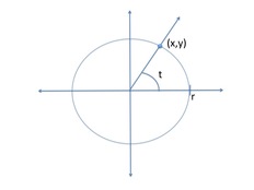
Figura 1. Círculo con centro en el origen y radio $r$.
Para graficar una curva que está definida usando ecuaciones paramétricas, computamos los valores de $x$ y $y$ para un conjunto de valores del parámetro. Por ejemplo, para $r = 2$, algunos de los valores son
| $t$ | $x$ | $y$ |
|---|---|---|
| $0$ | $2$ | $0$ |
| $\frac{\pi}{4}$ | $\frac{\sqrt{2}}{2}$ | $\frac{\sqrt{2}}{2}$ |
| $\frac{\pi}{2}$ | $0$ | $2$ |
Figura 2. Algunas coordenadas de los puntos $(x,y)$ del círculo con radio $r=2$ y centro en el origen.
Sesión de laboratorio:
En la introducción al tema de funciones viste que, tanto en matemáticas como en algunos lenguajes de programación, una función no puede devolver más de un resultado. En los ejercicios de esta experiencia de laboratorio practicarás cómo usar variables de referencia para poder obtener varios resultados de una función.
Ejercicio 1
En este ejercicio estudiarás la diferencia entre pase por valor y pase por referencia.
Instrucciones
Carga a Qt el proyecto
prettyPlothaciendo doble “click” en el archivoprettyPlot.proque se encuentra en la carpetaDocuments/eip/Functions-PrettyPlotsde tu computadora. También puedes ir ahttp://bitbucket.org/eip-uprrp/functions-prettyplotspara descargar la carpetaFunctions-PrettyPlotsa tu computadora.Configura el proyecto y ejecuta el programa marcando la flecha verde en el menú de la izquierda de la ventana de Qt Creator. El programa debe mostrar una ventana parecida a la Figura 3.
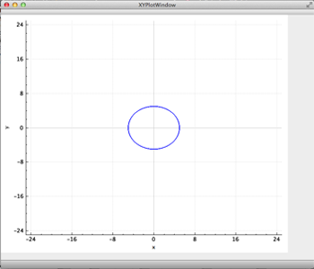
Figura 3. Gráfica de un círculo de radio 5 y centro en el origen desplegada por el programa PrettyPlot.
Abre el archivo
main.cpp(en Sources). Estudia la funciónillustrationy su invocación desde la funciónmain. Nota que las variablesargValueyargRefestán inicializadas a 0 y que la invocación aillustrationhace un pase por valor deargValuey un pase por referencia deargRef. Nota también que a los parámetros correspondientes enillustrationse les asigna el valor 1.Ejecuta el programa y observa lo que se despliega en la ventana
Application Output. Nota la diferencia entre el contenido las variablesargValueyargRefa pesar de que ambas tenían el mismo valor inicial y de que aparamValueyparamRefse les asignó el mismo valor. Explica por qué el contenido deargValorno cambia, mientras que el contenido deargRefcambia de 0 a 1.
Ejercicio 2
En este ejercicio practicarás la creación de una función sobrecargada.
Instrucciones
Estudia el código de la función
main()del archivomain.cpp. La líneaXYPlotWindow wCircleR5;crea el objetowCircleR5que será la ventana en donde se dibujará una gráfica, en este caso la gráfica de un círculo de radio 5. De manera similar se crean los objetoswCircleywButterfly. Observa el ciclofor. En este ciclo se genera una serie de valores para el ángulo $t$ y se invoca la funcióncircle, pasándole el valor de $t$ y las referencias a $x$ y $y$. La funcióncircleno devuelve valor pero, usando parámetros por referencia, calcula valores para las coordenadas $xCoord$ y $yCoord$ del círculo con centro en el origen y radio 5 y permite que la funciónmaintenga esos valores en las variablesx,y.Luego de la invocación, cada par ordenado $(x,y)$ es añadido a la gráfica del círculo por el método
AddPointToGraph(x,y). Luego del ciclo se invoca el métodoPlot(), que “dibuja” los puntos, y el métodoshow(), que muestra la gráfica. Los métodos son funciones que nos permiten trabajar con los datos de los objetos. Nota que cada uno de los métodos se escribe luego dewCircleR5, seguido de un punto. En una experiencia de laboratorio posterior aprenderás más sobre objetos y practicarás cómo crearlos e invocar sus métodos.La función
circleimplementada en el programa es muy restrictiva ya que siempre calcula los valores para las coordenadas $x$ y $y$ del mismo círculo: el círculo con centro en el origen y radio 5.Ahora crearás una función sobrecargada
circleque reciba como argumentos el valor del ángulo $t$, la referencia a las variables $x$ y $y$, y el valor para el radio del círculo. Invoca desdemain()la función sobrecargadacircleque acabas de implementar para calcular los valores de las coordenadas $x$ y $y$ del círculo con radio 15 y dibujar su gráfica. Grafica el círculo dentro del objetowCircle. Para esto, debes invocar desdemain()los métodosAddPointToGraph(x,y),Plotyshow. Recuerda que éstos deben ser precedidos porwCircle, por ejemplo,wCircle.show().
Ejercicio 3
En este ejercicio implantarás otra función para calcular las coordenadas de los puntos de la gráfica de una curva.
Instrucciones
Ahora crearás una función para calcular las coordenadas de los puntos de la gráfica que parece una mariposa. Las ecuaciones paramétricas para las coordenadas de los puntos de la gráfica están dadas por:
$$x=5\cos(t) \left[ \sin^2(1.2t) + \cos^3(6t) \right]$$ $$y= 10\sin(t) \left[ \sin^2(1.2t) + \cos^3(6t) \right].$$
Observa que ambas expresiones son casi iguales, excepto que una comienza con $5\cos(t)$ y la otra con $10\sin(t)$. En lugar de realizar el cómputo de $ \sin^2(1.2t) + \cos^3(6t)$ dos veces, puedes asignar su valor a otra variable $q$ y realizar el cómputo así:
$$q = \sin^2(1.2t) + \cos^3(6t)$$ $$x = 5 \cos(t)(q)$$ $$y = 10 \sin(t)(q).$$
Implementa la función
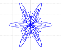
butterflyutilizando las expresiones de arriba, invoca la función desdemain()y observa la gráfica que resulta. Se supone que parezca una mariposa. Esta gráfica debe haber sido obtenida dentro de un objetoXYPlotWindowllamadowButterfly, invocando métodos de manera similar a como hiciste en el Ejercicio 2 para el círculo.
En [3] puedes encontrar otras ecuaciones paramétricas de otras curvas interesantes.
Entregas
Utiliza “Entrega” en Moodle para entregar el archivo main.cpp que contiene las funciones que implementaste, las invocaciones y cambios que hiciste en los ejercicios 2 y 3. Recuerda utilizar buenas prácticas de programación, incluir el nombre de los programadores y documentar tu programa.
Referencias
[1] http://mathbits.com/MathBits/CompSci/functions/UserDef.htm
[2] http://paulbourke.net/geometry/butterfly/
[3] http://en.wikipedia.org/wiki/Parametric_equation
Using functions in C++ - Pretty Plots
A good way to organize and structure computer programs is dividing them into smaller parts using functions. Each function carries out a specific task of the problem that we are solving.
You’ve seen that all programs written in C++ must contain the main function where the program begins. You’ve probably already used functions such as pow, sin, cos, or sqrt from the cmath library. Since in almost all of the upcoming lab activities you will continue using pre-defined functions, you need to understand how to work with them. In future exercises you will learn how to design and validate functions. In this laboratory experience you will invoke and define functions that compute the coordinates of the points of the graphs of some curves. You will also practice the implementation of arithmetic expressions in C++.
Objectives:
- Identify the parts of a function: return type, name, list of parameters, and body.
- Invoke pre-defined functions by passing arguments by value (“pass by value”), and by reference (“pass by reference”).
- Implement a simple overloaded function.
- Implement a simple function that utilizes parameters by reference.
- Implement arithmetic expressions in C++.
Pre-Lab:
Before you get to the laboratory you should have:
Reviewed the following concepts:
a. the basic elements of a function definition in C++.
b. how to invoke functions in C++.
c. the difference between parameters that are passed by value and by reference.
d. how to return the result of a function.
e. implement arithmetic expressions in C++.
f. use functions and arithmetic constants from the
cmathlibrary.g. a circle’s graph and equation.
Studied the concepts and instructions for the laboratory session.
Taken the Pre-Lab quiz that can be found in Moodle.
Functions
In mathematics, a function $f$ is a rule that is used to assign to each element $x$ from a set called domain, one (and only one) element $y$ from a set called range. This rule is commonly represented with an equation, $y=f(x)$. The variable $x$ is the parameter of the function and the variable $y$ will contain the result of the function. A function can have more than one parameter, but only one result. For example, a function can have the form $y=f(x_1,x_2)$ where there are two parameters, and for each pair $(a,b)$ that is used as an argument in the function, the function has only one value of $y=f(a,b)$. The domain of the function tells us the type of value that the parameter should have and the range tells us the value that the returned result will have.
Functions in programming languages are similar. A function has a series of instructions that take the assigned values as parameters and performs a certain task. In C++ and other programming languages, functions return only one result, as it happens in mathematics. The only difference is that a programming function could possibly not return any value (in this case the function is declared as void). If the function will return a value, we use the instruction return. As in math, you need to specify the types of values that the function’s parameters and result will have; this is done when declaring the function.
Function header:
The first sentence of a function is called the header and its structure is as follows:
type name(type parameter01, ..., type parameter0n)
For example,
int example(int var1, float var2, char &var3)
would be the header of the function called example, which returns an integer value. The function receives as arguments an integer value (and will store a copy in var1), a value of type float (and will store a copy in var2) and the reference to a variable of type char that will be stored in the reference variable var3. Note that var3 has a & symbol before the name of the variable. This indicates that var3 will contain the reference to a character.
Invoking
If we want to store the value of the example function’s result in a variable result (that would be of type integer), we invoke the function by passing arguments as follows:
result=example(2, 3.5, unCar);
Note that as the function is invoked, you don’t include the type of the variables in the arguments. As in the definition for the function example, the third parameter &var3 is a reference variable; what is being sent to the third argument when invoking the function is a reference to the variable unCar. Any changes that are made on the variable var3 will change the contents of the variable unCar.
You can also use the function’s result without having to store it in a variable. For example you could print it:
cout << "The result of the function example is:" << example(2, 3.5, unCar);
or use it in an arithmetic expression:
y=3 + example(2, 3.5, unCar);
Overloaded functions
Overloaded functions are functions that have the same name, but a different signature.
The signature of a function is composed of the name of the function, and the types of parameters it receives, but does not include the return type.
The following function prototypes have the same signature:
int example(int, int) ;
void example(int, int) ;
string example(int, int) ;
Note that each has the same name, example, and receives the same amount of parameters of the same type (int, int).
The following function prototypes have different signatures:
int example(int) ;
int elpmaxe(int) ;
Note that even though the functions have the same amount of parameters with the same type int, the name of the functions is different.
The following function prototypes are overloaded versions of the function example:
int example(int) ;
void example(char) ;
int example(int, int) ;
int example(char, int) ;
int example(int, char) ;
All of the above functions have the same name, example, but different parameters. The first and second functions have the same amount of parameters, but their arguments are of different types. The fourth and fifth functions have arguments of type char and int, but in each case are in different order.
In that last example, the function example is overloaded since there are 5 functions with different signatures but with the same name.
Values by default
Values by default can be assigned to the parameters of the functions starting from the first parameter to the right. It is not necessary to initialize all of the parameters, but the ones that are initialized should be consecutive: parameters in between two parameters cannot be left uninitialized. This allows calling the function without having to send values in the positions that correspond to the initialized parameters.
Examples of function headers and valid invocations:
Headers:
int example(int var1, float var2, int var3 = 10)Herevar3is initialized to 10.Invocations:
a.
example(5, 3.3, 12)This function call assigns the value 5 tovar1, the value 3.3 tovar2, and the value of 12 tovar3.b.
example(5, 3.3)This function call sends the values for the first two parameters and the value for the last parameter will be the value assigned by default in the header. That is, the values in the variables in the function will be as follows:var1will be 5,var2will be 3.3, andvar3will be 10.Header:
int example(int var1, float var2=5.0, int var3 = 10)Herevar2is initialized to 5 andvar3to 10.Invocations:
a.
example(5, 3.3, 12)This function call assigns the value 5 tovar1, the value 3.3 tovar2, and the value 12 tovar3.b.
example(5, 3.3)In this function call only the first two parameters are given values, and the value for the last parameter is the value by default. That is, the value forvar1within the function will be 5, that ofvar2will be 3.3, andvar3will be 10.c.
example(5)In this function call only the first parameter is given a value, and the last two parameters will be assigned values by default. That is,var1will be 5,var2will be 5.0, andvar3will be 10.
Example of a valid function header with invalid invocations:
Header:
int example(int var1, float var2=5.0, int var3 = 10)Invocation:
a.
example(5, , 10)This function call is invalid because it leaves an empty space in the middle argument.b.
example()This function call is invalid becausevar1was not assigned a default value. A valid invocation to the functionexampleneeds at least one argument (the first).
Examples of invalid function headers:
int example(int var1=1, float var2, int var3)This header is invalid because the default values can only be assigned starting from the rightmost parameter.int example(int var1=1, float var2, int var3=10)This header is invalid because you can’t place parameters without values between other parameters with default values. In this case,var2doesn’t have a default value butvar1andvar3do.
Parametric equations
Parametric equations allow us to represent a quantity as a function of one or more independent variables called parameters. In many occasions it is useful to represent curves using a set of parametric equations that express the coordinates of the points of the curve as functions of the parameters. For example, in your trigonometry course you should have studied that the equation of the circle of radius $r$ and centered at the origin has the following form:
$$x^2+y^2=r^2.$$
The points $(x,y)$ that satisfy this equation are the points that form the circle of radius $r$ and center at the origin. For example, the circle with $r=2$ and center at the origin has equation
$$x^2+y^2=4,$$
and its points are the ordered pairs $(x,y)$ that satisfy this equation. A parametric representation of the coordinates of the points in the circle of radius $r$ and center at the origin is:
$$x=r \cos(t)$$
$$y=r \sin(t),$$
where $t$ is a parameter that corresponds to the measure (in radians) of the positive angle with initial side that coincides with the positive part of the $x$-axis and terminal side that contains the point $(x,y)$, as it is illustrated in Figure 1.
Figure 1. Circle with center in the origin and radius $r$.
To plot a curve that is described by parametric equations, we compute the $x$ and $y$ values for a set of values of the parameter. For example, for $r=2$, some of the values are
| $t$ | $x$ | $y$ |
|---|---|---|
| $0$ | $2$ | $0$ |
| $\frac{\pi}{4}$ | $\frac{\sqrt{2}}{2}$ | $\frac{\sqrt{2}}{2}$ |
| $\frac{\pi}{2}$ | $0$ | $2$ |
Figure 2. Some coordinates for the points $(x,y)$ for the circle with radius $r=2$ and center in the origin.
Laboratory session:
In the introduction to the topic of functions you saw that in mathematics and in some programming languages, a function cannot return more than one result. In this laboratory experience’s exercises you will practice how to use reference variables to obtain various results from a function.
Exercise 1
In this exercise you will study the difference between pass by value and pass by reference.
Instructions
Load the project
prettyPlotin Qt by double clicking on the fileprettyPlot.proin the folderDocuments/eip/Functions-PrettyPlotsof your computer. You may also go tohttp://bitbucket.org/eip-uprrp/functions-prettyplotsto download the folderFunctions-PrettyPlotsto your computer.Configure the project and execute the program by clicking on the green arrow in the menu on the left side of the Qt Creator screen. The program should show a window similar to the one in Figure 3.
Figure 3. Graph of a circle with radius 5 and center in the origin displayed by the program PrettyPlot.
Open the file
main.cpp(in Sources). Study theillustrationfunction and how to call it from themainfunction. Note that the variablesargValueandargRefare initialized to 0 and that the function call forillustrationmakes a pass by value ofargValueand a pass by reference ofargRef. Also note that the corresponding parameters inillustrationare assigned a value of 1.Execute the program and observe what is displayed in the window
Application Output. Notice the difference between the content of the variablesargValueandargRefdespite the fact that both had the same initial value, and thatparamValueandparamRefwere assigned the same value. Explain why the content ofargValordoes not change, while the content ofargRefchanges from 0 to 1.
Exercise 2
In this exercise you will practice the creation of an overloaded function.
Instructions
Study the code in the
main()function in the filemain.cpp. The lineXYPlotWindow wCircleR5;creates awCircleR5object that will be the window where the graph will be drawn, in this case the graph of a circle of radius 5. In a similar way, the objectswCircleandwButterflyare created. Observe theforcycle. In this cycle a series of values for the angle $t$ is generated and the functioncircleis invoked, passing the value for $t$ and the references to $x$ and $y$. Thecirclefunction does not return a value, but using parameters by reference, it calculates the values for the coordinates $xCoord$ and $yCoord$ for the circle with center in the origin and radius 5, and allows themainfunction to have these values in thex,yvariables.After the function call, each ordered pair $(x,y)$ is added to the circle’s graph by the member function
AddPointToGraph(x,y). After the cycle, the member functionPlot()is invoked, which draws the points, and the member functionshow(), which displays the graph. The members functions are functions that allow use to work with and object’s data. Notice that each one of the member functions is written afterwCircleR5, followed by a period. In an upcoming laboratory experience you will learn more about objects, and practice how to create them and invoke their method functions.The
circlefunction implemented in the program is very restrictive since it always calculates the values for the coordinates $x$ and $y$ of the same circle: the circle with center in the origin and radius 5.Now you will create an overloaded function
circlethat receives as arguments the value of the angle $t$, the reference to the variables $x$ and $y$, and the value for the radius of the circle. Invoke the overloaded functioncirclethat you just implemented frommain()to calculate the values of the coordinates $x$ and $y$ for the circle with radius 15 and draw its graph. Graph the circle within thewCircleobject. To do this, you must invoke the method functionsAddPointToGraph(x,y),Plotandshowfrommain(). Remember that these should be preceded bywCircle, for example,wCircle.show().
Exercise 3
In this exercise you will implement another function to calculate the coordinates of the points in the graph of a curve.
Instructions
Now you will create a function to calculate the coordinates of the points of a graph that resembles a butterfly. The parametric equations for the coordinates of the points in the graph are given by:
$$x=5\cos(t) \left[ \sin^2(1.2t) + \cos^3(6t) \right]$$ $$y= 10\sin(t) \left[ \sin^2(1.2t) + \cos^3(6t) \right].$$
Observe that both expressions are almost the same, except that one starts with $5\cos(t)$ and the other with $10\sin(t)$. Instead of doing the calculation for $ \sin^2(1.2t) + \cos^3(6t)$ twice, you can assign its value to another variable $q$ and calculate it as such:
$$q = \sin^2(1.2t) + \cos^3(6t)$$ $$x = 5 \cos(t)(q)$$ $$y = 10 \sin(t)(q).$$
Implement the function
butterflyusing the expressions above, invoke the function inmain()and observe the resulting graph. It is supposed to look like a butterfly. This graph should have been obtained with aXYPlotWindowobject calledwButterfly, invoking method functions similar to how you did in Exercise 2 for the circle.
In [3] you can find other parametric equations from other interesting curves.
Deliverables
Use “Deliverables” in Moodle to hand in the file main() that contains the functions you implemented, the function calls and changes you made in exercises 2 and 3. Remember to use good programming techniques, include the name of the programmers involved and document your program.
References
[1] http://mathbits.com/MathBits/CompSci/functions/UserDef.htm